|
Many theories have been developed since the early 1900s
describing the heat and mass transfer phenomenon which
takes place in several types of atmospheric water cooling
devices. Most of these theories are based on sound engineering
principles. The cooling tower may be considered as a
heat exchanger in which water and air are in direct
contact with one another. There is no acceptable method
for accurately calculating the total contact surface
between water and air. Therefore, a "K" factor,
or heat transfer coefficient, cannot be determined directly
from test data or by known heat transfer theories. The
process is further complicated by mass transfer. Experimental
tests conducted on the specified equipment designs can
be evaluated using accepted and proven theories which
have been developed using dimensional analysis techniques.
These same basic methods and theories can be used for
thermal design and to predict performance at the operating
conditions other than the design point.
Many types of heat and mass
transfer devices defined the solution by theoretical
methods or dimensional analysis. Design data must be
obtained by the full-scale tests under the actual operating
conditions. Items such as evaporative condensers in
which an internal heat load is being applied, along
with water and air being circulated over the condenser
tubes in indefinable flow patterns, presents a problem
which cannot be solved directly by mathematical methods.
The boundary conditions have not been adequately defined
and the fundamental equations describing the variables
have not been written. Other devices such as spray ponds,
atmospheric spray towers, and the newer spray canal
systems have not been accurately evaluated solely by
mathematical means. This type of equipment utilizes
mixed flow patterns of water and air. Many attempts
have been made to correlate performance using "drop
theories", "cooling efficiency", number
of transfer units, all without proven results. Accurate
design data are best obtained by the actual tests over
a wide range of operating conditions with the specified
arrangement.
The development of cooling
tower theory seems to begin with Fitzgerald. The American
Society of Civil Engineers had asked Fitzerald to write
a paper on evaporation, and what had appeared to be
a simple task resulted in a 2 year investigation. The
result, probably in keeping with the time, is more of
an essay than a modern technical paper. Since the study
of Fitzgerald, many peoples like Mosscrop, Coffey &
Horne, Robinson, and Walker, etc. tried to develop the
theory.
1) Merkel Theory
|
The
early investigators of cooling tower theory grappled
with the problem presented by the dual transfer
of heat and mass. The Merkel theory overcomes
this by combining the two into a single process
based on enthalpy potential. Dr. Frederick Merkel
was on the faculty of the Technical College of
Dresden in Germany. He died untimely after publishing
his cooling tower paper. The theory had attracted
little attention outside of Germany until it was
discovered in German literature by H.B. Nottage
in 1938.
Cooling tower research
had been conducted for a number of years at University
of California at Berkley under the direction of
Professor L.K.M. Boelter. Nottage, a graduate
student, was assigned a cooling tower project
which he began by making a search of the literature.
He found a number of references to Merkel, looked
up the paper and was immediately struck by its
importance. It was brought to the attention of
Mason and London who were also working under Boelter
and explains how they were able to use the Merkel
theory in their paper.
Dr. Merkel developed
a cooling tower theory for the mass (evaporation
of a small portion of water) and sensible heat
transfer between the air and water in a counter
flow cooling tower. The theory considers the flow
of mass and energy from the bulk water to an interface,
and then from the interface to the surrounding
air mass. The flow crosses these two boundaries,
each offering resistance resulting in gradients
in temperature, enthalpy, and humidity ratio.
For the details for the derivation of Merkel theory,
refer to Cooling Tower Performance edited by Donald
Baker and the brief derivation is introduced here.
Merkel demonstrated that the total heat transfer
is directly proportional to the difference between
the enthalpy of saturated air at the water temperature
and the enthalpy of air at the point of contact
with water.
Q = K x S x (hw - ha)
where,
- Q = total heat transfer
Btu/h
- K = overall enthalpy
transfer coefficient lb/hr.ft2
- S = heat transfer
surface ft2. S equals to a x V, which
"a" means area of transfer surface
per unit of tower volume. (ft2/ft3),
and V means an effective tower volume (ft3).
- hw = enthalpy of
air-water vapor mixture at the bulk water temperature,
Btu/Lb dry air
- ha = enthalpy of
air-water vapor mixture at the wet bulb temperature,
Btu/Lb dry air
The water temperature
and air enthalpy are being changed along the fill
and Merkel relation can only be applied to a small
element of heat transfer surface dS.
dQ = d[K x S x (hw
- ha)] = K x (hw - ha) x dS
The heat transfer rate from water side is Q =
Cw x L x Cooling Range, where Cw = specific heat
of water = 1, L = water flow rate. Therefore,
dQ = d[Cw x L x (tw2 - tw1)] = Cw x L x dtw. Also,
the heat transfer rate from air side is Q = G
x (ha2 - ha1), where G = air mass flow rate Therefore,
dQ = d[G x (ha2 - ha1)] = G x dha.
Then, the relation of K x (hw - ha) x dS = G x
dha or K x (hw - ha) x dS = Cw x L x dtw are established,
and these can be rewritten in K x dS = G / (hw
- ha) x dha or K x dS / L = Cw / (hw - ha) x dtw.
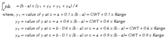
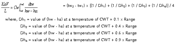
By integration,
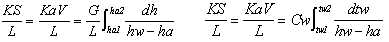
This basic heat transfer
equation is integrated by the four point Tchebycheff,
which uses values of y at predetermined values
of x within the interval a to b in numerically
evaluating the integral  .
The sum of these values of y multiplied by a constant
times the interval (b - a) gives the desired value
of the integral. In its four-point form the values
of y so selected are taken at values of x of 0.102673..,
0.406204.., 0.593796.., and 0.897327..of the interval
(b - a). For the determination of KaV/L, rounding
off these values to the nearest tenth is entirely
adequate. The approximate formula becomes: .
The sum of these values of y multiplied by a constant
times the interval (b - a) gives the desired value
of the integral. In its four-point form the values
of y so selected are taken at values of x of 0.102673..,
0.406204.., 0.593796.., and 0.897327..of the interval
(b - a). For the determination of KaV/L, rounding
off these values to the nearest tenth is entirely
adequate. The approximate formula becomes:
For the evaluation
of KaV/L,
|
2) Heat Balance
|
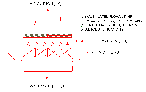
HEATin =
HEATout
WATER HEATin + AIR HEATin
= WATER HEATout + AIR HEATout
Cw L2 tw2 + G ha1
= Cw L1 tw1 + G ha2
Eq. 2-1
(The difference between L2 (entering
water flow rate) and L1 (leaving water
flow rate) is a loss of water due to the evaporation
in the direct contact of water and air. This evaporation
loss is a result of difference in the water vapor
content between the inlet air and exit air of
cooling tower. Evaporation Loss is expressed in
G x (w2 -w1) and is equal to L2
- L1. Therefore, L1 = L2
- G x (w2 -w1) is established.)
Let's replace the term
of L1 in the right side of Eq. 2-1
with the equation of L1 = L2
- G x (w2 -w1) and rewrite.
Then, Cw L2 tw2 + G ha1
= Cw [L2 - G x (w2 - w1)]
x tw1 + G ha2 is obtained.
This equation could be rewritten in Cw x L2
x (tw2 - tw1) = G x (ha2
- ha1) - Cw x tw1 x G x
(w2 - w1). In general, the
2nd term of right side is ignored to simplify
the calculation under the assumption of G x (w2
- w1) = 0.
Finally, the relationship
of Cw x L2 x (tw2 - tw1)
= G x (ha2 - ha1) is established
and this can be expressed to Cw x L x (tw2
- tw1) = G x (ha2 - ha1)
again. Therefore, the enthalpy of exit air, ha2
= ha1 + Cw x L / G x (tw2
- tw1) is obtained. The value of specific
heat of water is Eq. 2-1 and the term of tw2
(entering water temperature) - tw1
(leaving water temperature) is called the cooling
range.
Simply, ha2
= ha1 + L/G x Range Eq. 2-2
|
|


